v5.3.1 FIXED — The Framework + The Number + The Proofs
A. Al-Jabri — Z + C + A = 1 • From Sana'a to the Cosmos
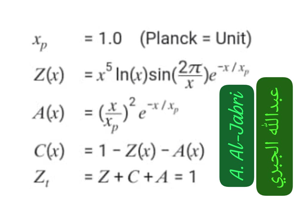
Zx = { xp=21, Z(x), A(x), C(x), Zt=1 } — Closure is the Essence
Before we speak about the number 21, we must first understand the framework that revealed it to us. Zx is not merely a name; it is an integrated mathematical system. It is what told us that the fundamental constant is 21 — not the other way around.
# ============================================================
#   jabri_visuals_v5.py
#   Generates Zx_Equations.png and Zx_Eq_figure.png
#   v5.0.1 — xp = 21 — equations above the plot
# ============================================================

!pip install matplotlib numpy --quiet 2>/dev/null

import numpy as np
import matplotlib.pyplot as plt
from matplotlib.patches import FancyBboxPatch
from matplotlib.gridspec import GridSpec
import matplotlib as mpl

mpl.rcParams['font.family'] = 'DejaVu Sans'

xp = 21.0

fig, ax = plt.subplots(figsize=(11, 7), dpi=200)
ax.set_xlim(0, 11); ax.set_ylim(0, 7); ax.axis('off')
fig.patch.set_facecolor('white')

eqs = [
    (6.1, r"$x_p \;=\; 21$", r"(Yemeni Constant)"),
    (5.0, r"$Z(x) \;=\; x^{-5}\,\ln(x)\,\sin\!\left(\frac{2\pi}{x}\right)\,e^{-x/x_p}$", ""),
    (3.9, r"$A(x) \;=\; \left(\frac{x}{x_p}\right)^{2}\,e^{-x/x_p}$", ""),
    (2.8, r"$C(x) \;=\; 1 \;-\; Z(x) \;-\; A(x)$", ""),
    (1.6, r"$Z_t \;=\; Z + C + A \;=\; 1$", ""),
]
for y, eq, note in eqs:
    ax.text(0, y, eq, fontsize=22, ha='left', va='center', color='#111')
    if note:
        ax.text(3.3, y, note, fontsize=13, ha='left', va='center', color='#666', style='italic')

for x0, txt in [(8.2, "A. Al-Jabri"), (9.4, "عبدالله الجبري")]:
    ax.add_patch(FancyBboxPatch((x0, 2.4), 0.85, 3.6, boxstyle="round,pad=0.1", linewidth=0, facecolor='#1e6b1e'))
    ax.text(x0 + 0.42, 4.2, txt, fontsize=15 if 'A.' in txt else 14, rotation=90, ha='center', va='center', color='#7fff7f', fontweight='bold' if 'A.' in txt else 'normal')

ax.text(5.5, 0.5, "Z + C + A = 1   •   From Sana'a to the Cosmos", fontsize=12, ha='center', color='#b5977a', fontweight='bold')
plt.tight_layout()
plt.savefig('Zx_Equations.png', dpi=200, bbox_inches='tight', facecolor='white')
plt.close()
print("✅ Zx_Equations.png")

fig = plt.figure(figsize=(12, 13), dpi=200)
fig.patch.set_facecolor('white')
gs = GridSpec(2, 1, height_ratios=[2.6, 4.0], hspace=0.12, left=0.06, right=0.97, top=0.97, bottom=0.05)

ax_eq = fig.add_subplot(gs[0])
ax_eq.set_xlim(0, 11); ax_eq.set_ylim(0, 7); ax_eq.axis('off')
eqs2 = [
    (6.1, r"$x_p \;=\; 21$", r"(Yemeni Constant)"),
    (5.0, r"$Z(x) \;=\; x^{-5}\,\ln(x)\,\sin\!\left(\frac{2\pi}{x}\right)\,e^{-x/x_p}$", ""),
    (3.9, r"$A(x) \;=\; \left(\frac{x}{x_p}\right)^{2}\,e^{-x/x_p}$", ""),
    (2.8, r"$C(x) \;=\; 1 \;-\; Z(x) \;-\; A(x)$", ""),
    (1.6, r"$Z_t \;=\; Z + C + A \;=\; 1$", ""),
]
for y, eq, note in eqs2:
    ax_eq.text(0, y, eq, fontsize=22, ha='left', va='center', color='#111')
    if note:
        ax_eq.text(3.3, y, note, fontsize=13, ha='left', va='center', color='#666', style='italic')

for x0, txt in [(8.2, "A. Al-Jabri"), (9.4, "عبدالله الجبري")]:
    ax_eq.add_patch(FancyBboxPatch((x0, 2.4), 0.85, 3.6, boxstyle="round,pad=0.1", linewidth=0, facecolor='#1e6b1e'))
    ax_eq.text(x0 + 0.42, 4.2, txt, fontsize=15 if 'A.' in txt else 14, rotation=90, ha='center', va='center', color='#7fff7f', fontweight='bold' if 'A.' in txt else 'normal')

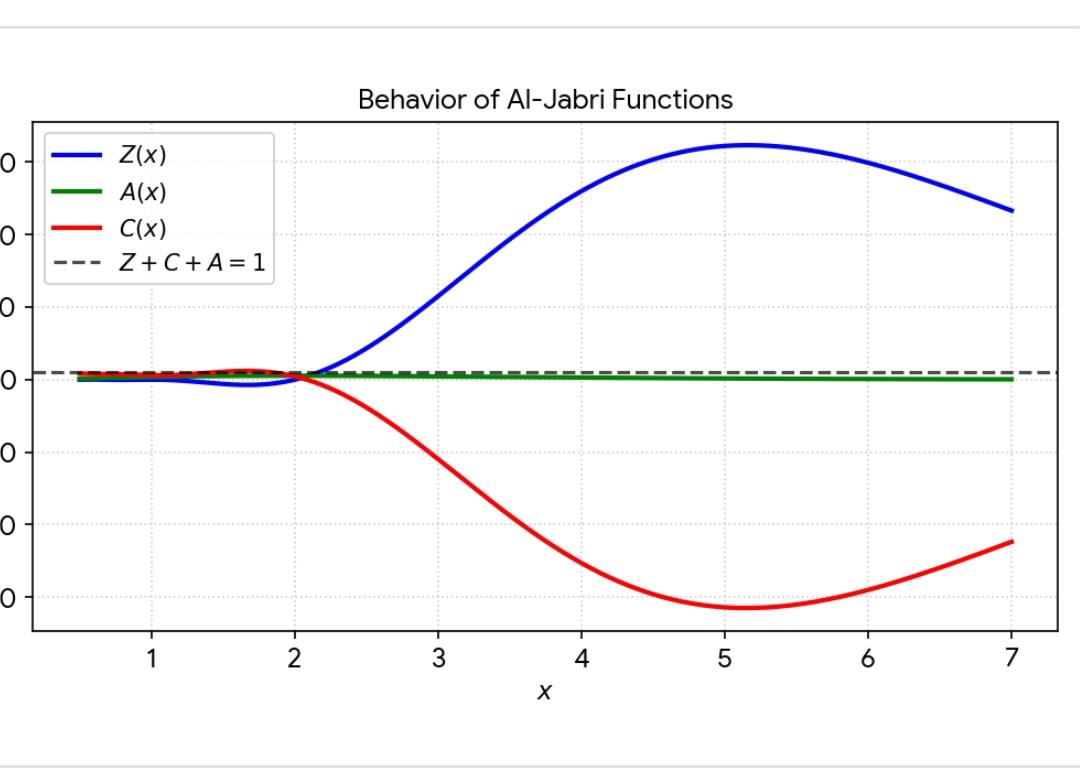
ax_plot = fig.add_subplot(gs[1])
x = np.linspace(0.5, 30, 5000)
Z = x**(-5.0) * np.log(x) * np.sin(2*np.pi/x) * np.exp(-x/xp)
A = (x/xp)**2 * np.exp(-x/xp)
C = 1.0 - Z - A

ax_plot.plot(x, Z, color='#1f4fd9', linewidth=2.2, label=r'$Z(x)$')
ax_plot.plot(x, A, color='#0f9b3f', linewidth=2.2, label=r'$A(x)$')
ax_plot.plot(x, C, color='#d92a2a', linewidth=2.2, label=r'$C(x)$')
ax_plot.axhline(1.0, color='#333', linestyle='--', linewidth=1.6, label=r'$Z + C + A = 1$')

ax_plot.set_xlabel(r'$x$', fontsize=15)
ax_plot.set_ylabel('Value', fontsize=15)
ax_plot.set_title(r'Behavior of Al-Jabri Functions  (v5.0.1,  $x_p = 21$)', fontsize=15, pad=12)
ax_plot.legend(fontsize=12, loc='upper right', framealpha=0.95)
ax_plot.grid(True, alpha=0.3, linestyle=':')
ax_plot.set_xlim(0.5, 30)
ax_plot.set_ylim(-1.6, 1.9)
ax_plot.axhline(0, color='#888', linewidth=0.7)

for n in [1, 2, 3, 4, 5]:
    xv = 2.0 / n
    if 0.5 <= xv <= 30:
        ax_plot.axvline(xv, color='#bbb', linestyle=':', linewidth=0.7, alpha=0.5)

plt.savefig('Zx_Eq_figure.png', dpi=200, bbox_inches='tight', facecolor='white')
plt.show()
print("✅ Zx_Eq_figure.png")
Having established that xp = 21 is the cornerstone of the Zx system, we now review the properties of this number.
| Property | Value / Representation | Reference |
|---|---|---|
| Definition | natural, odd, composite | zx-21-00 |
| Prime factorization | 21 = 3 × 7 (semiprime) | zx-21-01 zx-21-02 |
| Squarefree | yes | zx-21-03 |
| Divisors | 1, 3, 7, 21 | zx-21-04 |
| Number of divisors | τ(21) = 4 | zx-21-05 |
| Sum of divisors | σ(21) = 32 | zx-21-06 |
| Deficient | 1+3+7=11 < 21 | zx-21-07 |
| Euler's totient | φ(21) = 12 | zx-21-08 |
| Möbius function | μ(21) = 1 | zx-21-09 |
| Harshad number | 21 ÷ (2+1) = 7 | zx-21-10 |
| Binary | 10101₂ (palindromic) | zx-21-11 |
| Quaternary | 111₄ | zx-21-12 |
| Senary / Octal / Hex | 33₆ / 25₈ / 15₁₆ | zx-21-13 |
| Triangular | T₆ = 21 | zx-21-14 |
| Binomial coefficient | C(7,2) = 21 | zx-21-15 |
| Dice sum | 1+2+3+4+5+6 = 21 | zx-21-16 |
| Sums | 1²+2²+4² = 21 | zx-21-17 |
| Fibonacci | F₈ = 21 | zx-21-18 |
| Motzkin | M₅ = 21 | zx-21-19 |
| 21-gon | interior angle sum = 3420° | zx-21-20 |
| Number of diagonals | 189 | zx-21-21 |
| Pythagorean | 20²+21²=29² | zx-21-22 |
| Unhappy number | 21 → 5 → 25 → 29 → 85 → 89 → cycle | zx-21-23 |
| What it is not | not prime, not square, not cube, not perfect, not abundant | zx-21-24 |
| Feature of 42 | 42 = 2 × 21 (peak of A) | zx-21-25 |
# ============================================================
#   Count the zeros of the model function Z(x) at x = 0.5 + it
#   ⚠️ Note: these are zeros of the model Z, not zeros of the zeta function.
#      See Frame 1 §1 to distinguish Z(x) from ζ(s).
# ============================================================

import numpy as np

def Z_of_t(t, xp):
    x = complex(0.5, t)
    return np.exp(-x/xp) * (x**-5) * np.log(x) * np.sin(2*np.pi / x)

def count_zeros(xp, t_max=100, step=0.02):
    ts = np.arange(0.01, t_max, step)
    ims = np.array([Z_of_t(t, xp).imag for t in ts])
    zeros = 0
    for i in range(1, len(ims)):
        if ims[i-1]*ims[i] < 0:
            zeros += 1
    return zeros

print("xp | 0-60 | 0-100   (model-Z zeros)")
for xp in [5, 10, 18, 21, 50]:
    print(xp, count_zeros(xp, 60), count_zeros(xp, 100))
Methodology: we give the definition, explain, and prove... and leave the combinations and labels to the reader.
zx-xp-21
zx-Z-01
zx-A-01
zx-C-01
zx-Zt-01
For rigorous mathematical work: Frame 1 · Bridge · Frame 3 · Frame 4 · Status Dashboard.



Yemen - Sana'a - Safiya Hizyaz - near Al-Qasim Mosque - 67M4+MR
اليمن - صنعاء - صافية حزيز - جوار جامع القاسم - 67M4+MR
🗺️ Open in Google Maps